轴承异常检测

笔记本内容

简介 #

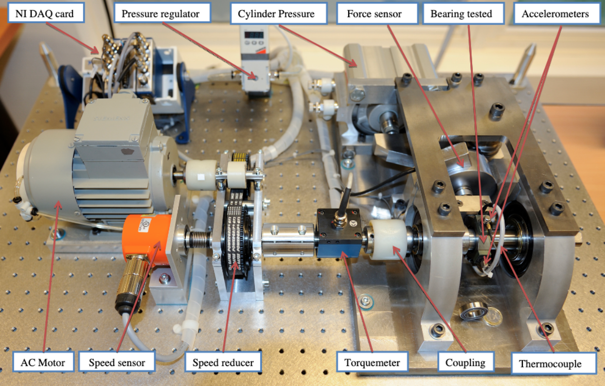
轴承是在机械设备中具有广泛应用的关键部件之一。由于过载，疲劳，磨损，腐蚀等原因，轴承在机器操作过程中容易损坏。事实上，超过50％的旋转机器故障与轴承故障有关。实际上，滚动轴承故障可能导致设备剧烈摇晃，设备停机，停止生产，甚至造成人员伤亡。一般来说，早期的轴承弱故障是复杂的，难以检测。因此，轴承状态的监测和分析非常重要，它可以发现轴承的早期弱故障，防止故障造成损失。最近，轴承的故障检测和诊断一直备受关注。在所有类型的轴承故障诊断方法中，振动信号分析是最主要和有用的工具之一。

import torch
import minetorch

import pandas as pd
import numpy as np
import seaborn as sns
import matplotlib.pyplot as plt

from sklearn.metrics import f1_score

batch_size = 8

DATA = '/home/featurize/data/train.csv'
TEST = '/home/featurize/data/test_data.csv'

train_df = pd.read_csv(DATA)
test_df = pd.read_csv(TEST)

对数据进行检视 #

训练集数据 #

1到6000是按时间序列连续采样的振动信号数值，每行数据为一个样本，共792条样本数据，第一列id字段为样本编号，最后一列label字段为标签数据，即轴承的工作状态，用数字0到9表示，其中

标签	轴承状态
0	正常状态
1	外圈故障、直径1类
2	内圈故障、直径1类
3	滚珠故障、直径1类
4	外圈故障、直径2类
5	内圈故障、直径2类
6	滚珠故障、直径2类
7	外圈故障、直径3类
8	内圈故障、直径3类
9	滚珠故障、直径3类

train_df.head(5)

	id	1	2	3	4	5	6	7	8	9	...	5992	5993	5994	5995	5996	5997	5998	5999	6000	label
0	1	0.563650	1.069229	-0.837759	-1.122021	0.433296	0.770755	-0.477153	-0.588421	0.455224	...	-0.050761	0.220506	0.036548	-0.097461	-0.084060	-0.007716	-0.049949	-0.018274	0.021523	7
1	2	0.061333	0.058830	0.056952	0.068634	0.073433	0.072390	0.042975	-0.007302	-0.026286	...	0.061333	0.107437	0.104516	0.063419	-0.014394	-0.048607	-0.009388	0.058830	0.129342	0
2	3	0.035736	0.010964	-0.164872	-0.167714	-0.125075	-0.104771	-0.016650	0.151471	0.137258	...	4.272044	-1.991455	-2.922208	1.937039	0.704156	-2.085667	0.203044	0.739892	-2.149829	9
3	4	-0.046700	0.060913	0.009340	-0.093400	-0.067817	0.022335	0.006091	-0.076751	-0.032893	...	0.095025	-0.000406	0.091776	0.074314	-0.082842	-0.110050	-0.028020	0.025990	-0.050355	9
4	5	0.162922	-0.377662	0.014457	0.565437	-0.203369	-0.511508	0.410961	0.228546	-0.515244	...	-0.093563	-0.263632	0.114517	0.209541	-0.184851	-0.075370	0.286211	0.005685	-0.223348	7

5 rows × 6002 columns

数据类别总体分布 #

sns.set()
sns.histplot(data=train_df.label, discrete=True);

轴承振动信号检视-时域 #

通过检视数据可以看到数据集中收集的是一个维度的振动信号，不同的标签对应的信号振幅应该有所不同。

f, ax = plt.subplots(5,2,figsize=(32,32))
state_list = [
    'Normal State',
    'Outer ring failure for 1st type diameter',
    'Inner ring failure for 1st type diameter',
    'Ball failure for 1st type diameter',
    'Outer ring failure for 2nd type diameter',
    'Inner ring failure for 2nd type diameter',
    'Ball failure for 2nd type diameter',
    'Outer ring failure for 3rd type diameter',
    'Inner ring failure for 3rd type diameter',
    'Ball failure for 3rd type diameter'
] 
for i in range(2):
    for j in range(5):
        ax[j][i].title.set_text(state_list[2*j+i])
        sns.lineplot(data=list(train_df[train_df.label==2*j+i].iloc[0][1:6001]), ax=ax[j][i]);

频域功率谱的分布 #

通过快速傅立叶变换对频域的功率谱做一个快速的可视化。

f, ax = plt.subplots(5,2,figsize=(32,32))
state_list = [
    'Normal State',
    'Outer ring failure for 1st type diameter',
    'Inner ring failure for 1st type diameter',
    'Ball failure for 1st type diameter',
    'Outer ring failure for 2nd type diameter',
    'Inner ring failure for 2nd type diameter',
    'Ball failure for 2nd type diameter',
    'Outer ring failure for 3rd type diameter',
    'Inner ring failure for 3rd type diameter',
    'Ball failure for 3rd type diameter'
] 
for i in range(2):
    for j in range(5):
        ax[j][i].title.set_text(state_list[2*j+i])
        fft = np.fft.fft(train_df[train_df.label==2*j+i].iloc[0][1:6001])
        sns.lineplot(data=(fft.real ** 2 - fft.imag ** 2), ax=ax[j][i]);

对数据进行分层抽样（Stratified Split） #

对数据进行分层抽样，按照1:9的比例分出对应的测试数据集和训练数据集。

from sklearn.model_selection import train_test_split
X_train, X_test, y_train, y_test = train_test_split(
    train_df.id, 
    train_df.label, 
    test_size=0.1, 
    random_state=42,
    stratify=train_df.label
)

整理数据格式(Data Cleaning) #

对原始数据进行清洗并且准备好神经网络接受的数据格式。

df_train = train_df.merge(X_train,on='id')
df_val = train_df.merge(X_test,on='id')

class BearingDataset(torch.utils.data.Dataset):
    def __init__(self, df):
        self.df = df

    def __getitem__(self, index: int):
        row = self.df.iloc[index]
        inputs = torch.tensor(row[1:6001]).unsqueeze(0)
        targets = torch.zeros(10)
        targets[int(row[-1])] = 1.
        
        return inputs.float(), targets
    def __len__(self):
        return len(self.df)

train_dataset = BearingDataset(
    df_train,
)

val_dataset = BearingDataset(
    df_val,
)

train_dataloader = torch.utils.data.DataLoader(
    train_dataset, num_workers=8, pin_memory=True, batch_size=batch_size)
val_dataloader = torch.utils.data.DataLoader(
    val_dataset, num_workers=8, pin_memory=True, batch_size=batch_size)

基于时域信号建立一维卷积神经网络 #

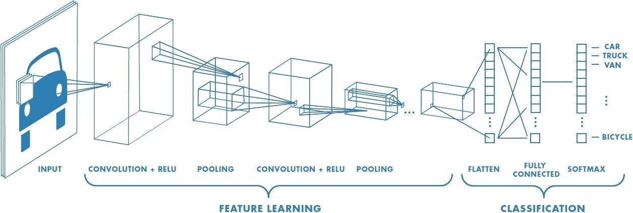
class Model(torch.nn.Module):
    def __init__(self):
        super(Model, self).__init__()
        self.conv = torch.nn.Conv1d(1, 16, 8, stride=2)
        self.conv1 = torch.nn.Conv1d(16, 16, 8, stride=2)
        self.conv2 = torch.nn.Conv1d(16, 64, 4, stride=2)
        self.conv2_ = torch.nn.Conv1d(64, 64, 4, stride=2)
        self.conv3 = torch.nn.Conv1d(64, 256, 4, stride=2)
        self.conv3_ = torch.nn.Conv1d(256, 256, 4, stride=2)
        self.conv4 = torch.nn.Conv1d(256, 512, 2, stride=2)
        self.conv4_ = torch.nn.Conv1d(512, 512, 2, stride=2)
        self.maxpool =  torch.nn.MaxPool1d(2)
        self.gap = torch.nn.AvgPool1d(1)
        self.dropout = torch.nn.Dropout(0.3)
        self.fc = torch.nn.Linear(512, 10)
        self.act = torch.nn.ReLU()

    def forward(self, x):
        x = self.conv(x)
        x = self.act(x)
        
        x = self.conv1(x)
        x = self.act(x)
        x = self.maxpool(x)
        
        x = self.conv2(x)
        x = self.act(x)
        x = self.conv2_(x)
        x = self.act(x)
        x = self.maxpool(x)
        
        x = self.conv3(x)
        x = self.act(x)
        x = self.conv3_(x)
        x = self.act(x)
        x = self.maxpool(x)

        x = self.conv4(x)
        x = self.act(x)
        x = self.conv4_(x)
        x = self.act(x)
        x = self.maxpool(x)

        x = self.gap(x)
        x = self.dropout(x)
        x = x.permute(0, 2, 1)
        x = self.fc(x).squeeze()

        return x

from minetorch.metrics import MultiClassesClassificationMetricWithLogic

class ClassificationMetric(MultiClassesClassificationMetricWithLogic):
    def before_epoch_start(self, epoch):
        self.predicts = np.array([]).astype(float)
        self.targets = np.array([]).astype(int)
        self.logits = np.array([]).astype(float)
    
    def after_val_iteration_ended(self, predicts, data, **ignore):
        predicts = (torch.sigmoid(predicts) > 0.5).int().detach().cpu().numpy() 
        targets = data[1].cpu().numpy()

        predicts = predicts.reshape([-1])
        targets = targets.reshape([-1])

        self.predicts = np.concatenate((self.predicts, predicts))
        self.targets = np.concatenate((self.targets, targets))
    
    def _accuracy(self):
        png_file = self.scalars(
            {"accuracy": (self.predicts == self.targets).sum() / len(self.predicts)},
            "accuracy",
        )
        if png_file:
            self.update_sheet(
                "accuracy", {"raw": png_file, "processor": "upload_image"}
            )
    '''
    def _roc(self):

        roc = roc_auc_score(self.targets, self.logits)
        png_file = self.scalars({'roc': roc}, 'roc')
        if png_file:
            self.update_sheet('roc', {'raw': png_file, 'processor': 'upload_image'})
    '''
    def _f1(self):
        score = f1_score(self.targets, self.predicts, average='macro')
        png_file = self.scalars({'f1': score}, 'f1')
        if png_file:
            self.update_sheet('f1', {'raw': png_file, 'processor': 'upload_image'})
    
    def after_epoch_end(self, val_loss, **ignore):
        #self._roc()
        self._f1()
        self.accuracy and self._accuracy()
        self.confusion_matrix and self._confusion_matrix()
        self.kappa_score and self._kappa_score()
        self.classification_report and self._classification_report()
        self.plot_confusion_matrix and self._plot_confusion_matrix(val_loss)

模型训练(Training) #

learning_rate = 1e-3
optimizer = torch.optim.AdamW(model.parameters(), lr=learning_rate, betas=(0.9, 0.999), eps=1e-08, weight_decay=1e-2, amsgrad=False)

model = Model()

def after_train_iteration_end(miner, *args, **kwargs):
    scheduler.step()
    miner.logger.info(f"current learning rate: {scheduler.get_last_lr()}")
    #miner.logger.info(f"current roc: {}")

def after_init(miner, *args, **kwargs):
    scheduler.step(miner.current_train_iteration)

miner = minetorch.Miner(
    code=os.getenv('CODE', f'baseline'),
    alchemistic_directory=os.getenv('ALCHEMISTIC_DIRECTORY', '/home/featurize/data/Bearing'),
    model=model.cuda(),
    optimizer=optimizer,
    train_dataloader=train_dataloader,
    val_dataloader=val_dataloader,
    max_epochs=30,
    in_notebook=True,
    loss_func=torch.nn.BCEWithLogitsLoss(),
    plugins=[ClassificationMetric()],
    #hooks={
    #    "after_train_iteration_end": after_train_iteration_end,
    #    "after_init": after_init
    #},
    trival=False,
    resume=False
)

miner.train()

ckpt = torch.load('/home/featurize/data/Bearing/baseline/models/latest.pth.tar')

F1 Score #

F1 Score是一种量测方法的精确度常用的指标，经常用来判断算法的精确度。目前在辨识、侦测相关的算法中经常会分别提到精确率（precision）和召回率（recall），F-score能同时考虑这两个数值，平衡的反映这个算法的精确度。

测试数据集表现 #

通过30轮的神经网络训练，模型已经收敛，在测试数据集上表现良好。

f, ax = plt.subplots(1,2, figsize=(20,5))
ax[0].title.set_text('F1 Score')
ax[1].title.set_text('Accuracy')
sns.lineplot(data=list(ckpt['drawer_state']['f1']['f1'].values()), ax=ax[0]);
sns.lineplot(data=list(ckpt['drawer_state']['accuracy']['accuracy'].values()), ax=ax[1]);

笔记本