实例
数据集
笔记本
镜像(公测)
笔记本

PyTorch 图像分类与图像分割中使用 CutMix
本实验主要是使用 CutMix 方法在管状腺癌、粘液腺癌、乳头状腺癌在病理图样上的识别,辅助现代医疗系统进行癌症诊断。
Dave上传于 5 years ago

笔记本内容
图像分类中如何使用 CutMix #

CutMix 是效果比较好的一类数据增强,常混迹于各大视觉比赛。
那么有小伙伴问了, CutMix 是什么呢?混砍?这我知道,我最近看的扫黑风暴里就有。。。也太暴力了。

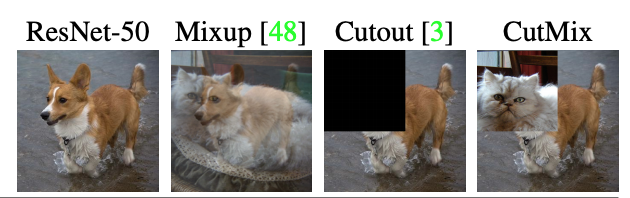
我说的是 CutMix: Regularization Strategy to Train Strong Classifierswith Localizable Features 这篇论文!
CutMix增强策略:
- 在训练图像中剪切和粘贴补丁,其中真实标签的混合与补丁的面积成正比。


# 如果自己工作区没有相关的包,请取消这一个 Cell 的注释进行安装
#%pip install segmentation_models_pytorch albumentations
#%pip install git+https://github.com/minetorch/minetorch.git
import os
import cv2
import torch
import minetorch
import random
import warnings
import numpy as np
import matplotlib.pyplot as plt
import pandas as pd
import seaborn as sns
import albumentations as albu
import segmentation_models_pytorch as smp
from sklearn.model_selection import train_test_split
from torch.utils.data import DataLoader, Dataset
from albumentations.pytorch import ToTensorV2
from albumentations import (Normalize, Compose)
from torch.optim.lr_scheduler import CosineAnnealingWarmRestarts
from minetorch.plugin import Plugin
from sklearn.metrics import cohen_kappa_score, confusion_matrix, classification_report
warnings.filterwarnings('ignore')# 配置
fold = 0 # KFold 策略中选择训练哪一个 fold
image_size = 512 # 图像需要 Resize 的尺寸
batch_size = 32 # 训练中的 batch_size, 32 是针对 V100-16G 的机器
ENCODER = 'tu-tf_efficientnet_b0' # Backbone 网络
Folder = '/home/featurize/JSH/' # 实验存放的目录(不需要手动创建)
MASK = '/home/featurize/data/train/train_mask' # mask 文件的存放目录
IMAGE = '/home/featurize/data/train/train_org_image' # 图片的存放目录# 读取 CSV 格式的标注文件
df = pd.read_csv('/home/featurize/data/train/train.csv')
df['image_path'] = '/home/featurize/data/train/train_org_image/'
df['mask_path'] = '/home/featurize/data/train/train_mask/'
train_df = df[df.fold != fold]
val_df = df[df.fold == fold]# CutMix 的切块功能
def rand_bbox(size, lam):
if len(size) == 4:
W = size[2]
H = size[3]
elif len(size) == 3:
W = size[0]
H = size[1]
else:
raise Exception
cut_rat = np.sqrt(1. - lam)
cut_w = np.int(W * cut_rat)
cut_h = np.int(H * cut_rat)
# uniform
cx = np.random.randint(W)
cy = np.random.randint(H)
bbx1 = np.clip(cx - cut_w // 2, 0, W)
bby1 = np.clip(cy - cut_h // 2, 0, H)
bbx2 = np.clip(cx + cut_w // 2, 0, W)
bby2 = np.clip(cy + cut_h // 2, 0, H)
return bbx1, bby1, bbx2, bby2# 一些比较基础的数据增广,包括水平翻转、垂直翻转等
def make_transforms(phase,mean=(0.485, 0.456, 0.406), std=(0.229, 0.224, 0.225)):
if phase == 'train':
transforms = albu.Compose(
[
albu.OneOf([
albu.HorizontalFlip(p=0.5),
albu.VerticalFlip(p=0.5),
albu.Transpose(p=0.5)
]),
albu.Resize(image_size,image_size, p=1),
albu.Normalize(mean=mean, std=std, p=1),
ToTensorV2(),
]
)
else:
transforms = albu.Compose(
[
albu.Resize(image_size, image_size, p=1),
albu.Normalize(mean=mean, std=std, p=1),
ToTensorV2(),
]
)
return transforms在这里定义 PyTorch Dataset 的时候就可以加入 CutMix 的操作了,在 Class 中用 “---” 分隔开了
# 定义 PyTorch 的 Dataset
class JSHDataset(Dataset):

    def __init__(self, df, transforms, train=False):
        self.df = df
        self.transforms = transforms
        self.train = train

    def __getitem__(self, idx):
        row = self.df.iloc[idx]
        fn = row.image_name
        # 读取图片数据
        image = cv2.imread(os.path.join(row['image_path'], fn))
        image = cv2.cvtColor(image, cv2.COLOR_BGR2RGB)
        image = cv2.resize(image, (1024, 1024), interpolation=cv2.INTER_LINEAR)
        # 读取 mask 数据
        masks = cv2.imread(os.path.join(row['mask_path'], fn), cv2.IMREAD_GRAYSCALE)/255
        masks = cv2.resize(masks, (1024, 1024), interpolation=cv2.INTER_LINEAR)
        # 读取 label
        label = torch.zeros(3)
        label[row.label] = 1
        # ------------------------------  CutMix  ------------------------------------------
        prob = 20  # 将 prob 设置为 0 即可关闭 CutMix
        if random.randint(0, 99) < prob and self.train:
            rand_index = random.randint(0, len(self.df) - 1)

            rand_row = self.df.iloc[rand_index]
            rand_fn = rand_row.image_name

            rand_image = cv2.imread(os.path.join(rand_row['image_path'], rand_fn))
            rand_image = cv2.cvtColor(rand_image, cv2.COLOR_BGR2RGB)
            rand_image = cv2.resize(rand_image, (1024, 1024), interpolation=cv2.INTER_LINEAR)

            rand_masks = cv2.imread(os.path.join(rand_row['mask_path'], rand_fn), cv2.IMREAD_GRAYSCALE)/255
            rand_masks = cv2.resize(rand_masks, (1024, 1024), interpolation=cv2.INTER_LINEAR)

            lam = np.random.beta(1,1)
            bbx1, bby1, bbx2, bby2 = rand_bbox(image.shape, lam)

            image[bbx1:bbx2, bby1:bby2, :] = rand_image[bbx1:bbx2, bby1:bby2, :]
            masks[bbx1:bbx2, bby1:bby2] = rand_masks[bbx1:bbx2, bby1:bby2]

            lam = 1 - ((bbx2 - bbx1) * (bby2 - bby1) / (image.shape[1] * image.shape[0]))

            rand_label = torch.zeros(3)
            rand_label[rand_row.label] = 1

            label = label * lam + rand_label * (1. - lam)
        # ---------------------------------  CutMix  ---------------------------------------
        # 应用之前我们定义的各种数据增广
        augmented = self.transforms(image=image, mask=masks)
        img, mask = augmented['image'], augmented['mask']
        return img, label, mask.unsqueeze(0)

    def __len__(self):
        return len(self.df)
# 使用 PyTorch 的 Dataloader 创建数据的生成器
trainset = JSHDataset(train_df, make_transforms('train'), train=True)
valset = JSHDataset(val_df, make_transforms('val'))
train_loader = DataLoader(
trainset,
batch_size=batch_size,
num_workers=8,
shuffle=True, # shuffle 是比较简单的打乱数据,如果在处理数据不均衡的数据集可以使用 sampler
pin_memory=True
)
val_loader = DataLoader(
valset,
batch_size=batch_size,
num_workers=8,
pin_memory=True
)sns.histplot()下面对原始数据和进行了 CutMix 操作的数据分别进行可视化。
random_list = [random.randint(0, len(trainset)-1) for i in range(5)]
f, ax = plt.subplots(2, 5, figsize=(14,4))
for i in range(5):
    img, _, mask = trainset.__getitem__(random_list[i])
    ax[0][i].imshow(
        torch.clip(img.permute(1,2,0), 0, 1)
    );
    ax[1][i].imshow(
        torch.clip(mask.permute(1,2,0), 0, 1)
    );

# 使用了 CutMix 之后的数据进行可视化,可以明显的看到数据中的“补丁”
random_list = [random.randint(0, len(trainset)-1) for i in range(5)]
f, ax = plt.subplots(2, 5, figsize=(14,4))
for i in range(5):
    img, _, mask = trainset.__getitem__(random_list[i])
    ax[0][i].imshow(
        torch.clip(img.permute(1,2,0), 0, 1)
    );
    ax[1][i].imshow(
        torch.clip(mask.permute(1,2,0), 0, 1)
    );

# 模型配置
ENCODER_WEIGHTS = 'imagenet'
ACTIVATION = None
DEVICE = 'cuda'
n_class = 1

# 创建分类的 head
aux_params=dict(
    pooling='avg',             # one of 'avg', 'max'
    activation=None,           # activation function, default is None
    classes=3,                 # define number of output labels
)

# 创建分割的 head 同时载入模型预训练权重
model = smp.FPN(
    ENCODER,
    classes=n_class,
    encoder_weights=ENCODER_WEIGHTS,
    activation=ACTIVATION,
    aux_params=aux_params
).cuda()

# 学习率、优化器、
learning_rate = 3e-5
optimizer = torch.optim.AdamW(model.parameters(), lr=learning_rate, betas=(0.9, 0.999), eps=1e-08, amsgrad=False)
# 创建前向传播
bce_loss = torch.nn.BCEWithLogitsLoss().cuda()
def forward_fn(trainer, data):
images, labels, masks = data
images, labels, masks = images.cuda(), labels.cuda(), masks.cuda()
mask, label = model(images)
loss = bce_loss(label, labels) + 3*bce_loss(mask, masks)
return (label, mask), loss# 这是 Minetorch 的一个可视化指标的插件,我们对分割的 Pixel Accuracy 和分类的 Accuracy 进行了记录
class MultiClassesSegmentationMetricWithLogic(Plugin):
"""MultiClassesClassificationMetric
This can be used directly if your loss function is torch.nn.CrossEntropy
"""
def __init__(self,
accuracy_s=True,
accuracy_c=True,
metric=True,
sheet_key_prefix=''):
super().__init__(sheet_key_prefix)
self.accuracy_s = accuracy_s
self.accuracy_c = accuracy_c
self.metric = metric
def before_init(self):
self.create_sheet_column('accuracy_s', 'Accuracy_s')
self.create_sheet_column('accuracy_c', 'Accuracy_c')
def before_epoch_start(self, epoch):
self.tpc, self.fpc, self.fnc, self.tnc = 0, 0, 0, 0
self.tps, self.fps, self.fns, self.tns = 0, 0, 0, 0
self.acc_s, self.acc_c, self.metric = 0, 0, 0
def after_val_iteration_ended(self, predicts, data, **ignore):
predicts_c = torch.sigmoid(predicts[0]).detach().cpu().numpy()
targets = data[1].detach().cpu().numpy()
self.tpc += (((predicts_c>0.5) == 1) * (targets == 1)).sum()
self.fpc += (((predicts_c>0.5) == 1) * (targets == 0)).sum()
self.fnc += (((predicts_c>0.5) == 0) * (targets == 1)).sum()
self.tnc += (((predicts_c>0.5) == 0) * (targets == 0)).sum()
predicts_s = torch.sigmoid(predicts[1]).detach().cpu().numpy()
targets = data[2].detach().cpu().numpy()
self.tps += (((predicts_s>0.5) == 1) * (targets == 1)).sum()
self.fps += (((predicts_s>0.5) == 1) * (targets == 0)).sum()
self.fns += (((predicts_s>0.5) == 0) * (targets == 1)).sum()
self.tns += (((predicts_s>0.5) == 0) * (targets == 0)).sum()
def after_epoch_end(self, val_loss, **ignore):
self.acc_s = float(self.tps + self.tns) / float(self.tps + self.fps + self.fns + self.tns+1e-12)
self.acc_c = float(self.tpc + self.tnc) / float(self.tpc + self.fpc + self.fnc + self.tnc+1e-12)
self.metric = 0.7 * self.acc_s + 0.3 * self.acc_c
self.accuracy_s and self._accuracy_s()
self.accuracy_c and self._accuracy_c()
self.metric and self._metric()
def _accuracy_s(self):
png_file = self.scalars(
{'accuracy_s': (self.acc_s)}, 'accuracy_s'
)
if png_file:
self.update_sheet('accuracy_s', {'raw': png_file, 'processor': 'upload_image'})
def _accuracy_c(self):
png_file = self.scalars(
{'accuracy_c': (self.acc_c)}, 'accuracy_c'
)
if png_file:
self.update_sheet('accuracy_c', {'raw': png_file, 'processor': 'upload_image'})
def _metric(self):
png_file = self.scalars(
{'metric': (self.metric)}, 'metric'
)
if png_file:
self.update_sheet('metric', {'raw': png_file, 'processor': 'upload_image'})
# 创建实验目录
if not os.path.isdir(Folder):
    os.mkdir(Folder)
# 训练器的配置
miner = minetorch.Miner(
code=os.getenv('CODE', f'fold-{fold}'),
alchemistic_directory=os.getenv('ALCHEMISTIC_DIRECTORY', f'{Folder}{ENCODER}-cutmix-{image_size}'),
model=model,
forward=forward_fn,
optimizer=optimizer,
train_dataloader=train_loader,
val_dataloader=val_loader,
max_epochs=100,
in_notebook=True,
loss_func=None,
amp=True,
plugins=[MultiClassesSegmentationMetricWithLogic()],
trival=False,
resume=False
)# 开始训练
miner.train()下面就是本次试验的结果了,我们一起来看一下 #
实验一:正常训练 #
f, axs = plt.subplots(1, 2, figsize=(14, 14))
axs[0].set_axis_off()
axs[1].set_axis_off()

axs[0].imshow(cv2.imread('/home/featurize/JSH/tu-tf_efficientnet_b0-512/fold-0/graphs/loss.png'));
axs[1].imshow(cv2.imread('/home/featurize/JSH/tu-tf_efficientnet_b0-512/fold-0/graphs/metric.png'));
实验二:增加了概率为 20% 的 CutMix 操作 #
f, axs = plt.subplots(1, 2, figsize=(14, 14))
axs[0].set_axis_off()
axs[1].set_axis_off()

axs[0].imshow(cv2.imread('/home/featurize/JSH/tu-tf_efficientnet_b0-cutmix-512/fold-0/graphs/loss.png'));
axs[1].imshow(cv2.imread('/home/featurize/JSH/tu-tf_efficientnet_b0-cutmix-512/fold-0/graphs/metric.png'));
把两个实验的 Loss 画到一张图上来对比一下。
可以清楚的看到 CutMix 操作在同样训练参数的情况下对 Validation 的 Loss 效果更优。
以上就是 CutMix 在图像分类以及分割当中的应用,请小伙伴们参考,如有错误也请大佬指正。
normal = torch.load('/home/featurize/JSH/tu-tf_efficientnet_b0-512/fold-0/models/latest.pth.tar')
cutmix = torch.load('/home/featurize/JSH/tu-tf_efficientnet_b0-cutmix-512/fold-0/models/latest.pth.tar')

normal = list(normal['drawer_state']['loss']['val'].values())[5:21]
cutmix = list(cutmix['drawer_state']['loss']['val'].values())[5:21]

f, ax = plt.subplots()
ax.set_title('Validation Loss')

ax.plot(np.linspace(5,20,16), normal);
ax.plot(np.linspace(5,20,16), cutmix);
plt.legend(['efficientnet-b0', 'efficientnet-b0 + CutMix(p=0.2)']);

评论(0条)